 |
 |
|||||
|
|
|
|
|
|
|
|
| A part of the National Science Foundation Scientific
Database Initiative Grant IRI 9116849 Last updated on April 5th, 2001 |
 |
|
| Scalability
Test Demo This experiment is to test the performance of our sequence matching algorithm with a large set of sequence data set. Since it is difficult to obtain a large set of sequence dataset, we shall take a small yet meaningful sequence dataset and transform into a large data set as describe in the following: |
|
1. Data set transformation The data set contains 20 patients and each patient has 3 lung images taken at different time. To transform this set of sequence images into a large set of image sequences for testing the scalability of our sequence matching algorithm, we divided each lung image into 96 sub-areas, thus making 96 sequences of length 3 for each patient. Thus the 20 patient image sequences were transformed into 1920 sequences with a length of 3 for each sequence. We extracted the following 7 features from each of the transformed images (represented as a sub area of the original image):
These features as well their corresponding feature values were provided by Dr. Matthew Brown of the Radiology Department, School of Medicine of UCLA. As a result, we have the following data set :
|
|
2. Pre-processing and Index construction
We applied the normalization for each dimension so that all dimensions have equal importance (weight). Without normalization, the features whose values are larger than the other features have more influence in determining the similarity of any two sequences. In our data set, the first feature (percentage of voxels) has the value around 10 while the third feature (standard deviation of gray level) has the value around 100. Therefore, without normalization, the third feature has influence roughly ten times larger than that of the first feature. Next, we built a TAH from the set of the elements from the normalized data sequences. Then we use the TAH to convert the normalized element sequence into a symbol sequence where symbol corresponds to the leaf node of the element in the TAH. Finally, we build the suffix tree from the set of symbol sequences. |
|
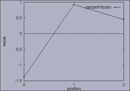
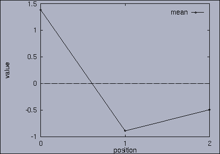
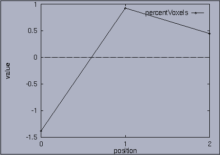
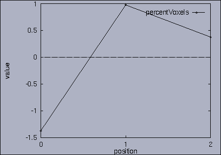
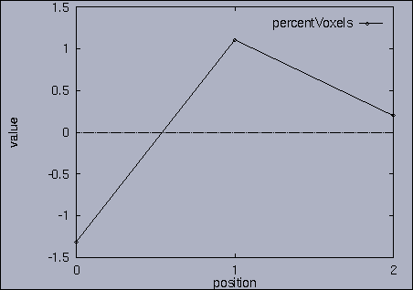
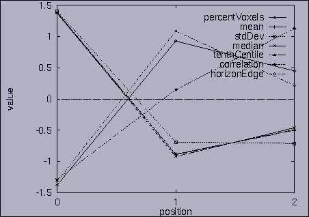
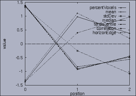
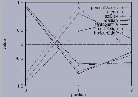
3. Query processing To submit a query, we first make a query file where we specify the features of interest and their relative weights as well as a query sequence itself. A query sequence can be displayed graphically using the following utility: % drawQry qryFile [dimension] By specifying the dimension number, we can see the changing pattern of a specific feature graphically. If the dimension number is "1", the first feature (in this scalability test, it is "percentage of voxels") is drawn as a line graph. And, if the dimension number is "2", the second feature (it is "mean of gray level") is drawn, and so on. If the "dimension" is not specified, all features are drawn together. |
|
|
|
|
|
|
|
|
|
|
| For executing a query, we use either one of the following commands:
% java SS_range datFile qryFile distanceTolerance % java SS_nn datFIle qryFile numAnswers The first one is for range queries and the second one is for nearest
neighbor queries. Both commands give a set of answers sorted by the
distances from the query sequence. To allow sequences to be stretched or
compressed along the time axis, the distance of any two (sub)sequences is
computed by the multi-dimensional time warping distance function. Let X[0]
denote the first element of the sequence X and Rest(X) denote the
subsequence of X containing all the elements of X except for the first
element. Then, the multi-dimensional time warping distance of two sequences
X and Y is defined as follows: Here, Dbase(X[0],Y[0]) represents the weighted city-block distance between X[0] and Y[0]. Each answer returned by our query processing method is represented like the following: "seqName startingOffset endingOffset distance" "datFile" is the name of a data file, which stores all data sequences in ascii format. "seqName", "startingOffset", and "endingOffset" indicates a subsequence of the "seqName" including all the elements in positions of "startingOffset" through "endingOffset". The distance is the weighted distance between the data sequence "seqName" with that of the query sequence. "nearest-neighbor.log" shows the 50 answers as shown in the following table:
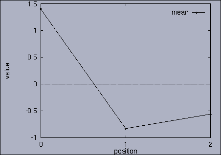
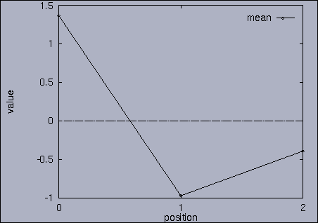
The best answer is "mseq1 0 2 0.00". mseq1 has the distance 0 since it is the exact query sequence. The next best answer is "mseq11 0 2 1.75". The third best answer is "mseq2 0 2 2.91". Their results are shown in snapshots 4,5,and 6. | ||||||||||||||||||||||||||||||||||||||||||||||||||||||||||||||||||||||||||||||||||||||||||||||||||||||||||||||||||||||||||||||||||||||||||||||||||||||||||||||||||||||||||||||||||||||||||||||||||||||||
|
|
||||||||||||||||||||||||||||||||||||||||||||||||||||||||||||||||||||||||||||||||||||||||||||||||||||||||||||||||||||||||||||||||||||||||||||||||||||||||||||||||||||||||||||||||||||||||||||||||||||||||
|
|
|
|
|
|
|
|
|
|
|
|
|
|
|
|
|
|
|
|
|
|
| Conclusion This scalability test reveals that our indexing method shows reasonable query processing performance even in large sequence databases. With 2000 sequences whose average length is 3, the response time for the queries of finding 50 similar answers was about 80 seconds. The response time increases linearly as the number of data sequences grows. The increase rate, however, is much smaller than that of sequential scanning method. (For more detailed information, the interested reader should refer to the ICDE 2000 paper) |
|
|
|
| Return to the previous KMeD page |
